用pytorch实现基于LSTM的循环神经网络。
涉及函数详解 class torch.nn.LSTM(args,*kwargs)
参数说明:
input_size: 输入的特征维度
output_size: 输出的特征维度
num_layers: 层数(注意与时序展开区分)
bidirectional: 如果为True,为双向LSTM。默认为False
LSTM的输入:input,$(h_0,c_0)$
input(seq_len,batch,input_size): 包含输入特征的tensor,注意输入是tensor。
$h_0$(num_layers $\cdot$ num_directions,batch,hidden_size): 保存初始化隐藏层状态的tensor
$c_0$(num_layers $\cdot$ num_directions,batch,hidden_size): 保存初始化细胞状态的tensor
LSTM的输出: output,$(h_n,c_n)$
output(seq_len, batch, hidden_size * num_directions): 保存RNN最后一层输出的tensor
$h_n$(num_layers * num_directions,batch,hidden_size): 保存RNN最后一个时间步隐藏状态的tensor
$c_n$(num_layers * num_directions,batch,hidden_size): 保存RNN最后一个时间步细胞状态的tensor
1
2
3
4
5
6
7
import torch.nn import torch lstm = nn.LSTM(embedding_dim,hidden_dim) #实例化一个LSTM单元,该单元输入维度embedding_dim,输出维度为hidden_dim input = Variable(torch.randn(seq_len,1,embedding_dim)) # 输入input应该是三维的,第一维度是seq-length,也就是多个词构成的一句话;第二维度为1,不用管;第三个维度是一个词的词嵌入维度,即embedding_dim h0 = Variable(torch.randn(1,1,hidden_dim)) c0 = Variable(torch.randn(1,1,hidden_dim)) lstm_out,hidden = lstm(input,(h0,c0))
class torch.nn.Linear() 1 class torch.nn.Linear(in_features,out_features,bias = True)
作用:对输入数据做线性变换。$y = Ax+b$
参数:
in_features:每个输入样本的大小
out_features: 每个输出样本的大小
bias: 默认值为True。是否学习偏置。
形状:
输入: (N,in_features)
输出: (N,out_features)
变量:
weights: 可学习的权重,形状为(in_features,out_features)
bias: 可学习的偏置,形状为(out_features)
1
2
3
4
m = nn.Linear(20,30) input = torch.randn(128,20) output = m(input) print(output)
先看个小例子 用pytorch实现LSTM,先实例化一个LSTM单元,再给出tensor类型的输入数据inputs及初始隐藏状态hidden = $(h_0,c_0)$。值得注意的是,LSTM单元的输入inputs必须是三维的,第一维是seq-length,即一句话,元素是词。第二维是mini-batch,从来不用,设为1即可。第三维是embedding-size,即一个词向量。
1
2
3
4
5
6
import torch import torch.nn as nn lstm = nn.LSTM(4,3) #实例化一个LSTM单元,单元输入维度是4,输出维度是3 inputs = [torch.randn(1,5) for _ in range(5)] #产生输入inputs。为tensor序列。 hidden = (torch.randn(1,1,3),torch.randn(1,1,3)) #初始化隐藏状态
做好三步准备:实例化一个LSTM单元,准备好inputs,初始化隐藏状态hidden。我们就可以计算LSTM单元的输出了。
1
2
3
for x in inputs: lstm_out,hidden = lstm(x.view(1,1,-1),hidden) #x.view(1,1,-1)将tensor整形为三维。前面说过LSTM单元的输入必须是三维的。 print(lstm_out,hidden)
接下来,将整个序列送入LSTM单元:
1
2
3
4
inputs = torch.cat(inputs).view(len(inputs),1,-1) #将整个序列连接为tensor,并整形为三维。 hidden = (torch.randn(1,1,3),torch.randn(1,1,3)) #清楚隐藏状态 lstm_out,hidden = lstm(inputs,hidden) print(lstm_out,hidden)
我们可以看到:
lstm_out 中包含了序列所有的隐藏状态。
hidden 中包含了最后一个时间步的隐藏状态和细胞状态。可以作为下个时间步LSTM单元的输入参数,继续输入序列或反向传播。
用lstm做词性标注 先准备训练数据:
1
2
3
4
5
6
7
8
9
10
11
12
13
14
15
train_data = [ ("The dog ate the apple".split(), ["DET", "NN", "V", "DET", "NN"]), ("Everybody read that book".split(), ["NN", "V", "DET", "NN"]) ] # 词汇表字典 word_to_ix = {} for sent,tags in train_data: for word in sent: if word not in word_to_ix: word_to_ix[word] = len(word_to_ix) # 标签集字典 tag_to_ix = {"DET": 0, "NN": 1, "V": 2} EMBEDDING_DIM = 6 HIDDEN_DIM = 6
构建LSTM模型:
1
2
3
4
5
6
7
8
9
10
11
12
class LSTMtagger(nn.Module): def __init__(self,embedding_dim,hidden_dim,vocab_size,tagset_size): super(LSTMtagger,self).__init__() self.hidden_dim = hidden_dim self.word_embeddings = nn.Embedding(vocab_size,embedding_dim) #随机初始化词向量表,是神经网络的参数 self.lstm = nn.LSTM(embedding_dim,hidden_dim) #实例化一个LSTM单元,单元输入维度是embedding_dim,输出维度是hidden_dim self.hidden2tag = torch.Linear(hidden_dim,tagset_size) #线性层从隐藏状态空间映射到标签空间 def forward(self,sentence): embeds = self.word_embeddings(sentence) #查询句子的词向量表示。输入应该是二维tensor。 lstm_out,hidden = self.lstm(embeds.view(len(sentence),1,-1)) tag_space = self.hidden2tag(lstm_out.view(len(sentence),-1)) tag_scores = F.log_softmax(tag_space)
训练模型
1
2
3
4
5
6
7
8
9
10
11
12
13
14
15
16
17
18
19
20
21
22
23
24
25
26
27
28
29
30
31
32
33
34
35
36
37
model = LSTMtagger(EMBEDDING_DIM,HIDDEN_DIM,len(word_to_ix),len(tag_to_ix)) loss_function = nn.NLLLoss() optimizer = optim.SGD(model.parameters(),lr = 0.1) def prepare_sequence(seq,to_ix): idxs = [to_ix[w] for w in seq] return torch.tensor(idxs,dtype = torch.long) # 在训练模型之前,看看模型预测结果 with torch.no_grad(): inputs = prepare_sequence(train_data[0][0],word_to_ix) tag_scores = model(inputs) print(tag_scores) predict = np.argmax(tag_scores,axis = 1) print(predict) for epoch in range(300): for sentence,tags in train_data: # step 1:pytorch会累积梯度,要清楚所有variable的梯度。 model.zero_grad() # step 2:准备好数据,变成tensor sentence_in = prepare_sequence(sentence,word_to_ix) targets = prepare_sequence(tags,tag_to_ix) # step 3:得到输出 tag_scores = model(sentence_in) # step4: 计算loss loss = loss_function(tag_scores,targets) # step5: 计算loss对所有variable的梯度 loss.backward() # step6: 单步优化,根据梯度更新参数 optimizer.step() # 模型训练后,看看预测结果 with torch.no_grad(): inputs = prepare_sequence(train_data[0][0],word_to_ix) tag_scores = model(inputs) print(tag_scores) predict = np.argmax(tag_scores,axis = 1) print(predict)
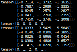
输出结果为:
我们可以看到,训练之后的预测序列为 [0,1,2,0,1]也就是[“DET”, “NN”, “V”, “DET”, “NN”]
参考链接
最后更新时间:2019-07-22 09:01:59